4 Between-Subjects Designs
The semnova() function can also be used with between-subjects factors and covariates. The between argument takes a vector of between-subjects factors (i.e., grouping variables). We estimate the same manifest model as in the very first example with the additional between-subjects factor sex. Using the between argument will cause semnova to estimate a multi-group model:
fit_btw <- semnova(
    data = reading_manifest,
    id = "id",
    dv = "re_fix_time",
    within = c("grade", "sentence"),
    between = "sex"
)

summary(fit_btw)
## Main and Interaction Effects:
## Chisq df Pr(>Chisq)
## Intercept 1.505 1 0.220
## grade 354.755 2 <2e-16 ***
## sentence 381.882 1 <2e-16 ***
## grade:sentence 84.370 2 <2e-16 ***
## sex 0.192 1 0.661
## grade:sex 1.969 2 0.374
## sentence:sex 1.800 1 0.180
## grade:sentence:sex 1.959 2 0.376
## ---
## Signif. codes: 0 '***' 0.001 '**' 0.01 '*' 0.05 '.' 0.1 ' ' 1When including between-subjects effects, hypothesis tests correspond to Type III sums of squares in ANOVA. Type III sums of squares do not take unbalanced group sizes into account as apposed to average effects (e.g., Gräfe et al., 2022). Tests for average effects remain work in progress and may be included in future releases.
Main and interaction effects for the within-subjects factors are again significant. Main and interaction effects involving the between-subjects factor sex are non-significant indicating that no differences exist across genders.
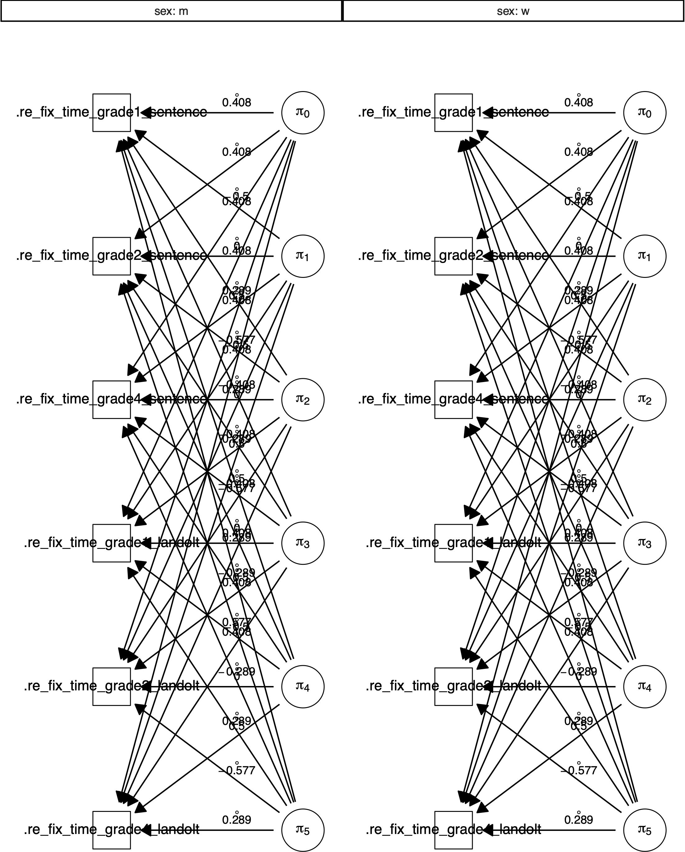
Figure 4.1: Path diagram created by plot(fit_btw) for a \(2 \times 3 \times 2\) (sentence \(\times\) grade \(\times\) sex) mixed design design with the manifest dependent variable re-fixation time.
4.1 Latent Variables
4.1.1 Measurement Model
The multi-group approach can also be used with latent variables. The command is identical to the previous purely within-subjects example that includes latent variables, except for the additional between argument.
fit_btw_latent <- semnova(
    data = reading_latent,
    id = "id",
    dv = "dv",
    indicator = "indicator",
    equal_resid_cov = list("ini_land_pos", "fix_count"),
    between = "sex",
    within = c("grade", "sentence"),
    missing = "fiml"
)

summary(fit_btw_latent)
## Fit measures:
##
## Chisq(280) = 693.254, p = 0
## CFI = 0.833
## TLI = 0.817
## RMSEA = 0.105 [0.095, 0.115]
##
## ##############################
##
## Main and Interaction Effects:
## Chisq df Pr(>Chisq)
## Intercept 0.035 1 0.852
## grade 765.984 2 <2e-16 ***
## sentence 651.753 1 <2e-16 ***
## grade:sentence 310.771 2 <2e-16 ***
## sex 0.253 1 0.615
## grade:sex 1.446 2 0.485
## sentence:sex 1.469 1 0.226
## grade:sentence:sex 1.993 2 0.369
## ---
## Signif. codes: 0 '***' 0.001 '**' 0.01 '*' 0.05 '.' 0.1 ' ' 1The model fit is again not very good. Hypothesis tests show the same pattern as for the model using only the manifest variable re-fixation time. A path diagram of the model is shown in Figure 4.2.
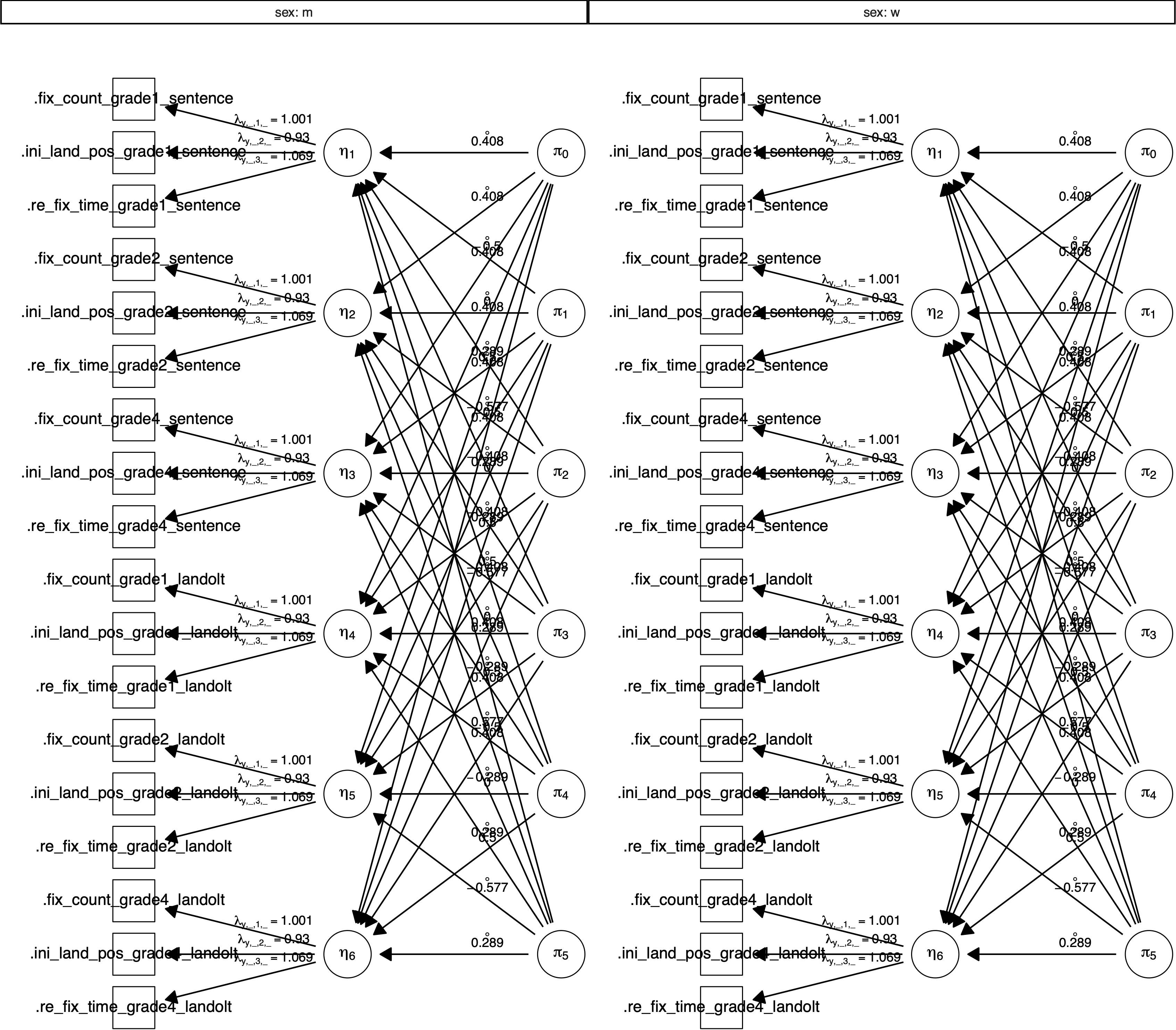
Figure 4.2: Path diagram created by plot(fit_btw_latent) for a \(2 \times 3 \times 2\) (sentence \(\times\) grade \(\times\) sex) mixed design with the latent dependent variable reading ability measured by the three manifest variables re-fixation time, initial landing position and fixation count.
4.1.2 Measurement Invariance
Measurement invariance must also be tested across groups. In order to be able to compare means between groups, strong measurement invariance is needed (i.e., equal loadings and intercepts between groups). This can be done by sequentially comparing models that assume different degrees of measurement invariance (i.e., configural, weak, strong, or strict). The invariance_between argument can be set to "configural", "weak", "strong", or "strict".
fit_btw_latent_configMI <- semnova(
    data = reading_latent,
    id = "id",
    dv = "dv",
    indicator = "indicator",
    equal_resid_cov = list("ini_land_pos", "fix_count"),
    between = "sex",
    within = c("grade", "sentence"),
    missing = "fiml",
    invariance_between = "configural"
)

fit_btw_latent_weakMI <- semnova(
    data = reading_latent,
    id = "id",
    dv = "dv",
    indicator = "indicator",
    equal_resid_cov = list("ini_land_pos", "fix_count"),
    between = "sex",
    within = c("grade", "sentence"),
    missing = "fiml",
    invariance_between = "weak"
)

fit_btw_latent_strongMI <- semnova(
    data = reading_latent,
    id = "id",
    dv = "dv",
    indicator = "indicator",
    equal_resid_cov = list("ini_land_pos", "fix_count"),
    between = "sex",
    within = c("grade", "sentence"),
    missing = "fiml",
    invariance_between = "strong"
)

fit_btw_latent_strictMI <- semnova(
    data = reading_latent,
    id = "id",
    dv = "dv",
    indicator = "indicator",
    equal_resid_cov = list("ini_land_pos", "fix_count"),
    between = "sex",
    within = c("grade", "sentence"),
    missing = "fiml",
    invariance_between = "strict"
)

anova(
    fit_btw_latent_configMI,
    fit_btw_latent_weakMI,
    fit_btw_latent_strongMI,
    fit_btw_latent_strictMI
)
## Chi-Squared Difference Test
##
## Df AIC BIC Chisq Chisq diff Df diff Pr(>Chisq)
## fit_btw_latent_configMI 272 5636.4 6016.6 686.14
## fit_btw_latent_weakMI 276 5633.9 5999.8 691.62 5.487 4 0.2408
## fit_btw_latent_strongMI 280 5627.5 5979.1 693.25 1.630 4 0.8034
## fit_btw_latent_strictMI 298 5677.5 5964.5 779.30 86.043 18 7.356e-11
##
## fit_btw_latent_configMI
## fit_btw_latent_weakMI
## fit_btw_latent_strongMI
## fit_btw_latent_strictMI ***
## ---
## Signif. codes: 0 '***' 0.001 '**' 0.01 '*' 0.05 '.' 0.1 ' ' 1The fit of the first model is not very good. These results are in line with the results for the latent model from the previous examples. However, we can see that weak and strong measurement invariance explain the data equally well as compared to configural measurement invariance. The strict measurement invariance model, however, differs in terms of fit as compared to the other three models.