3 Within-Subjects Designs
For the first code example, we use the two within-subjects factors sentence type and grade from the motivating example with the manifest variable re-fixation time neglecting the between-subjects factor sex. The function semnova() offers a range of features and is used to estimate the first model:
fit <- semnova(
    data = reading_manifest,
    id = "id",
    dv = "re_fix_time",
    within = c("grade", "sentence")
)
The function takes at least three arguments: id is a character vector of variables that uniquely identify the subjects, dv takes the name of the dependent variable, and data takes a data set in the long format (also called narrow format). Furthermore, within takes a vector of variables containing experimental within-subjects factors.
The next command is the summary() function which we use to extract the results from the model:
summary(fit)## Main and Interaction Effects:
## Chisq df Pr(>Chisq)
## Intercept 4.711 1 0.03 *
## grade 832.066 2 <2e-16 ***
## sentence 515.317 1 <2e-16 ***
## grade:sentence 234.919 2 <2e-16 ***
## ---
## Signif. codes: 0 '***' 0.001 '**' 0.01 '*' 0.05 '.' 0.1 ' ' 1The function prints hypothesis tests for each of the main and interaction effects. By default, the output contains a Wald test for the effects, future releases will include more statistics such as the likelihood ratio test and an approximate \(F\)-test. The factor grade has three levels and the test consequently has two degrees of freedom. All tests are highly significant, leading to the rejection of the null hypothesis and suggesting that the re-fixation time is neither constant across grade nor across the sentence types.
We can further use the print() function to print parameter estimates for each of the freely estimated model parameters. The following output is truncated after seven rows due to the large number of parameters.
print(fit)##
##
## parameter est se pvalue
## ------------------- ----------- ---------- ----------
## alpha_{pi,1,1} -0.0677313 0.0312067 0.0299760
## sigma_{pi,1,1,1}^2 0.1636084 0.0178511 0.0000000
## sigma_{pi,1,2,1}^2 -0.0354949 0.0116314 0.0022760
## sigma_{pi,1,3,1}^2 -0.0165968 0.0082027 0.0430381
## sigma_{pi,1,4,1}^2 -0.0275617 0.0138830 0.0471122
## sigma_{pi,1,5,1}^2 0.0400701 0.0143246 0.0051533
## sigma_{pi,1,6,1}^2 0.0063447 0.0101050 0.5300847
## alpha_{pi,2,1} -0.7971504 0.0279478 0.0000000
## sigma_{pi,2,2,1}^2 0.1312214 0.0143174 0.0000000
## sigma_{pi,2,3,1}^2 -0.0249054 0.0075061 0.0009066
## sigma_{pi,2,4,1}^2 0.0258745 0.0124476 0.0376466
## sigma_{pi,2,5,1}^2 -0.0147721 0.0125781 0.2402218
## sigma_{pi,2,6,1}^2 0.0255615 0.0092517 0.0057293
## alpha_{pi,3,1} 0.0681849 0.0200307 0.0006640
## sigma_{pi,3,3,1}^2 0.0674062 0.0073546 0.0000000
## sigma_{pi,3,4,1}^2 0.0096321 0.0088372 0.2757335
## sigma_{pi,3,5,1}^2 0.0341557 0.0093566 0.0002618
## sigma_{pi,3,6,1}^2 0.0085963 0.0065123 0.1868360
## alpha_{pi,4,1} -0.7699475 0.0339175 0.0000000
## sigma_{pi,4,4,1}^2 0.1932668 0.0210871 0.0000000
## sigma_{pi,4,5,1}^2 -0.0326321 0.0154091 0.0341988
## sigma_{pi,4,6,1}^2 -0.0105359 0.0110000 0.3381557
## alpha_{pi,5,1} 0.5290506 0.0345798 0.0000000
## sigma_{pi,5,5,1}^2 0.2008881 0.0219187 0.0000000
## sigma_{pi,5,6,1}^2 -0.0264462 0.0113687 0.0200060
## alpha_{pi,6,1} -0.0470649 0.0249530 0.0592762
## sigma_{pi,6,6,1}^2 0.1046057 0.0114134 0.0000000The plot() function further plots a path diagram for the model. shows two path diagrams. Per default, the diagram will only show regression arrows and measurement model arrows (see Figure 3.1). The what argument can be used to also draw intercepts, variances, covariances, residual variances and residual covariances (see Figure 3.2).
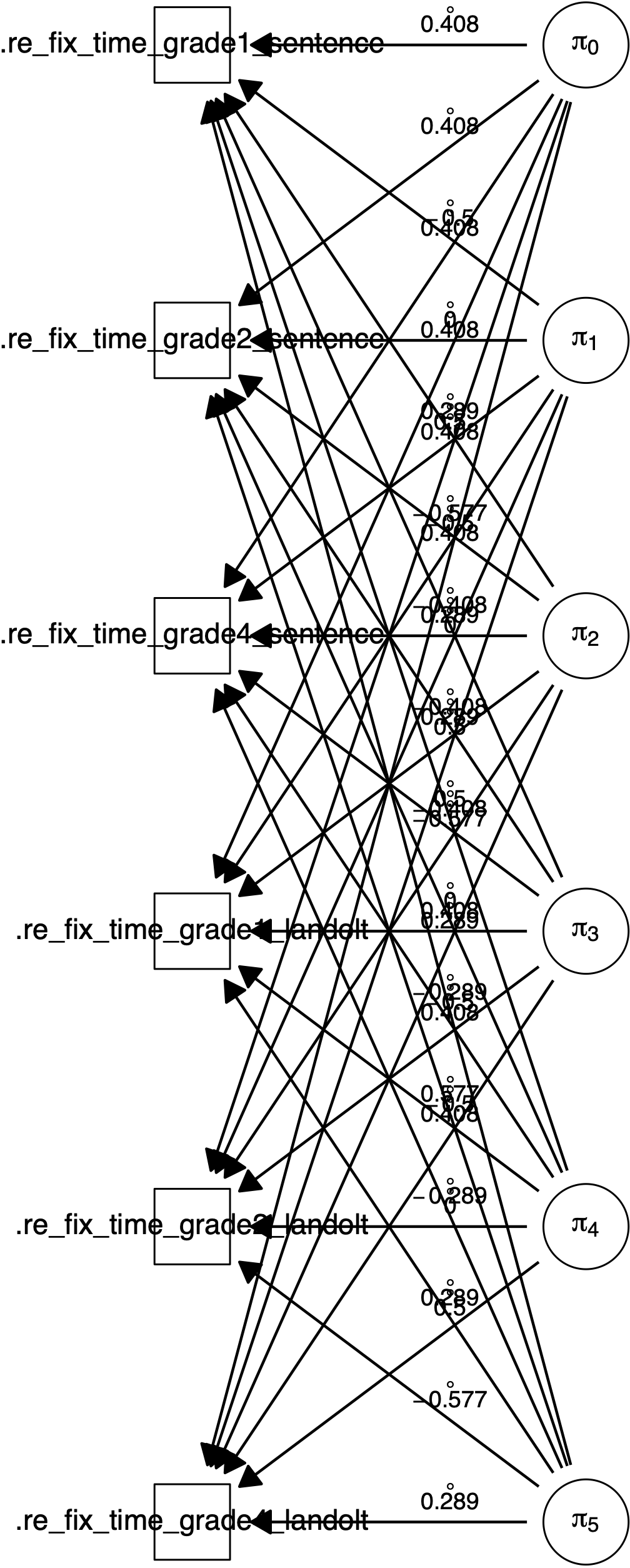
Figure 3.1: Path diagram for a \(2 \times 3\) (sentence \(\times\) grade) within-subjects design with the manifest dependent variables re-fixation time. Created by plot(fit).
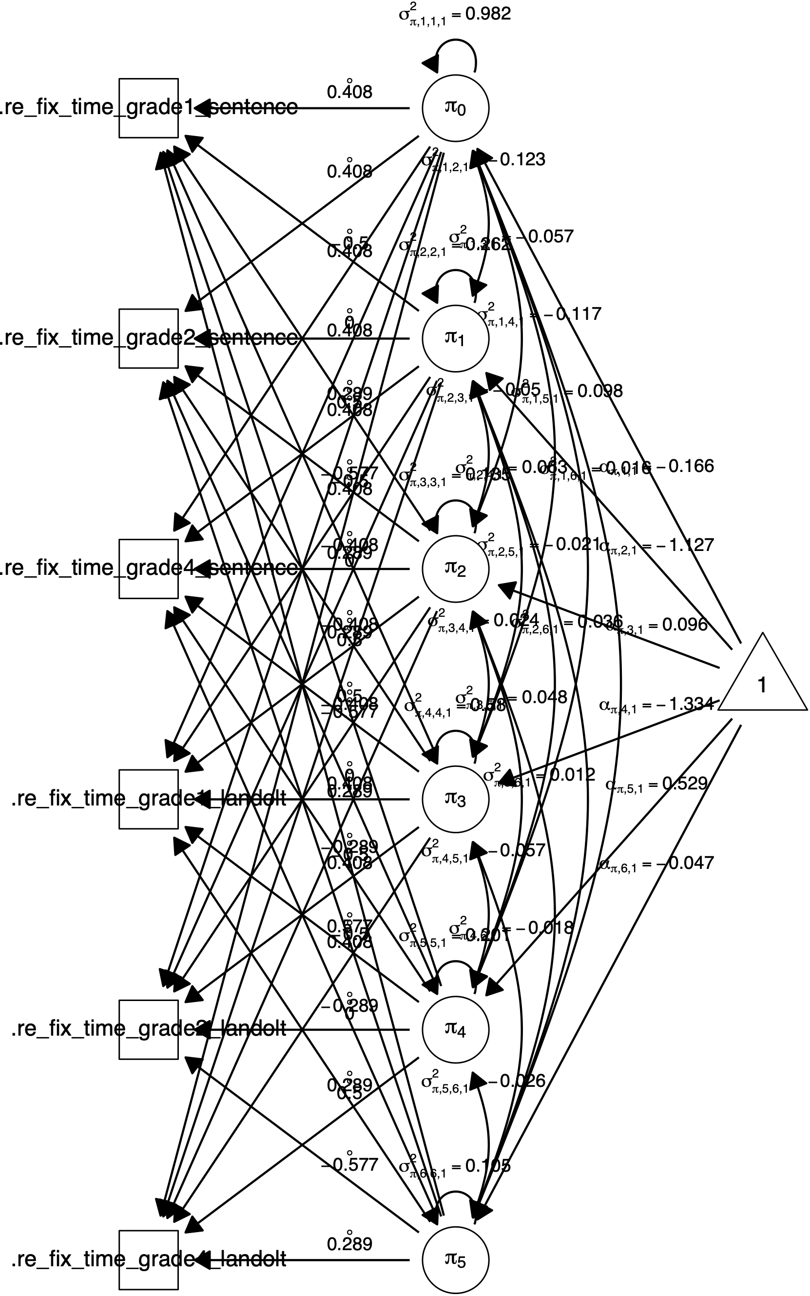
Figure 3.2: Path diagram for a \(2 \times 3\) (sentence \(\times\) grade) within-subjects design with the manifest dependent variables re-fixation time. Created by plot(fit, what = "all").
3.1 Sphericity
The next example shows how semnova can be used to test for sphericity as described in Chapter 4 “Understanding, Testing, and Relaxing Sphericity of Repeated Measures ANOVA with Manifest and Latent Variables Using SEM” (Langenberg, 2022). The semnova() function offers the sphericity argument to impose sphericity for a set of experimental factors. By default, the argument is FALSE. The argument can also take a list of vectors of experimental factors. Each vector describes an effect consisting of factor names (i.e., variable names) for which sphericity is to be assumed. For the factor grade, the code looks as follows:
## Chi-Squared Difference Test
##
##               Df    AIC    BIC  Chisq Chisq diff Df diff Pr(>Chisq)
## fit            0 1494.6 1579.0  0.000
## fit_sph_grade  2 1521.1 1599.2 30.518     30.518       2  2.361e-07 ***
## ---
## Signif. codes:  0 '***' 0.001 '**' 0.01 '*' 0.05 '.' 0.1 ' ' 1
All arguments are the same as for the previous example except for the sphericity argument. The factor grade has three levels and thus two effect variables. This command will force the variances of the effect variables \(\pi_1\) and \(\pi_2\) to be equal and their covariance to be zero. The anova() function can compare multiple models. Comparing a model with unconstrained covariance matrix to a model that imposes sphericity yields a formal test for sphericity.
The test is significant, suggesting that sphericity cannot be assumed. That is, either the variances of the effect variables are unequal, or the covariance is not zero. Thus, univariate test statistics cannot be used and multivariate tests should be preferred (e.g., Lane, 2016). The test presents an alternative to the often-used Mauchly’s sphericity test (Mauchly, 1940).
The same test can be performed for the interaction of grade and sentence type because the effect consists of the two contrast variables \(\pi_4\) and \(\pi_5\) (i.e., the effect has two degrees of freedom):
fit_sph_grade_sentence <- semnova(
    data = reading_manifest,
    id = "id",
    dv = "re_fix_time",
    within = c("grade", "sentence"),
    sphericity = list(c("grade", "sentence"))
)

anova(fit, fit_sph_grade_sentence)
## Chi-Squared Difference Test
##
## Df AIC BIC Chisq Chisq diff Df diff Pr(>Chisq)
## fit 0 1494.6 1579 0.000
## fit_sph_grade_sentence 2 1513.9 1592 23.262 23.262 2 8.884e-06 ***
## ---
## Signif. codes: 0 '***' 0.001 '**' 0.01 '*' 0.05 '.' 0.1 ' ' 1The sphericity argument is now a list consisting of a character vector with two elements indicating that sphericity is to be assumed for the interaction effect of grade and sentence type. The test is again significant and sphericity does not hold for the interaction effect.
Lastly, it is possible to perform an omnibus test for sphericity. This test assumes sphericity for all effects that have two or more degrees of freedom. Note that the variances and covariances of, and between, effect variables belonging to different effects (e.g., the contrast variable \(\pi_1\) from the main effect of grade and the contrast variable \(\pi_4\) from the interaction effect) are not constrained and are freely estimated. The following test will have four degrees of freedom (i.e., the sum of the degrees of freedom of the separate tests).
fit_sph_all <- semnova(
    data = reading_manifest,
    id = "id",
    dv = "re_fix_time",
    within = c("grade", "sentence"),
    sphericity = list("grade", c("grade", "sentence"))
)

anova(fit, fit_sph_all)
## Chi-Squared Difference Test
##
## Df AIC BIC Chisq Chisq diff Df diff Pr(>Chisq)
## fit 0 1494.6 1579 0.000
## fit_sph_all 4 1536.1 1608 49.511 49.511 4 4.567e-10 ***
## ---
## Signif. codes: 0 '***' 0.001 '**' 0.01 '*' 0.05 '.' 0.1 ' ' 1The test is also significant. We can use the test as an omnibus test to avoid multiple testing issues such as cumulative Type 1 errors. If the test is non-significant, we can assume sphericity for all effects and proceed with the more strict model which may give us a gain in statistical power (e.g., Lane, 2016; Muller & Barton, 1989). However, if the test is significant, we cannot say which of the effects violates the assumption and we have to perform both sphericity tests separately.
Note that, instead of list(c("grade", "sentence"), "grade"), the sphericity argument can also be set to TRUE imposing sphericity for all of the effects. The argument can also take a formula such as FALSE ~ grade:sentence which is equivalent to using list(c("grade", "sentence")). The formula reads as “do not assume sphericity (FALSE) except (~) for the interaction effect of sentence and grade (sentence:grade)”.
3.2 Latent Variables
3.2.1 Measurement Model
The semnova() function can also incorporate latent variables. The input looks the same as for the very first example. Only this time, the indicator argument is provided, which takes the variable name of the data set that contains the names of the indicators. The variable named “indicator” from the example data set contains the values re_fix_dur, "ini_land_pos" and "fix_count". Furthermore, the argument equal_resid_cov can be used to allow for residual covariances between the indicators. Residual covariances between indicators are forced to be equal across experimental conditions. For instance, the covariances between the manifest variables of re-fixation time will be the same across all of the six experimental conditions. In this example, we use the variables re-fixation time, initial landing position and fixation count to form a latent variable that measures reading ability. By default, semnova uses a congeneric measurement model with strong measurement invariance and the effect-code identification scheme (Little et al., 2006) to set the scale for the latent variables (see also Langenberg, 2022, sec. 2.4.1 “Defining the Model”). We will further use full information maximum likelihood for this example because of several missing values by using missing = "fiml". Full information maximum likelihood is implemented in the lavaan package and the argument is passed on to lavaan.
fit_latent <- semnova(
    data = reading_latent,
    id = "id",
    dv = "dv",
    indicator = "indicator",
    equal_resid_cov = list("ini_land_pos", "fix_count"),
    within = c("grade", "sentence"),
    missing = "fiml"
)

summary(fit_latent)
## Fit measures:
##
## Chisq(138) = 461.551, p = 0
## CFI = 0.861
## TLI = 0.845
## RMSEA = 0.094 [0.084, 0.103]
##
## ##############################
##
## Main and Interaction Effects:
## Chisq df Pr(>Chisq)
## Intercept 0.416 1 0.519
## grade 1432.334 2 <2e-16 ***
## sentence 1037.801 1 <2e-16 ***
## grade:sentence 607.323 2 <2e-16 ***
## ---
## Signif. codes: 0 '***' 0.001 '**' 0.01 '*' 0.05 '.' 0.1 ' ' 1The output now contains a section for fit indices in addition to hypothesis tests. The hypothesis tests are again significant. The fit is not very good but the example is intended to demonstrate the basic usage of the software package. The fit can be poor for several reasons. For instance, measurement invariance across the experimental conditions may not hold. This assumption will be examined in the next section. As a consequence, we should be very cautious when interpreting parameter estimates and hypothesis tests.
In complex latent variables models, negative (residual) variances are also an issue. This can happen if the variances of the latent variables are very small as compared to residual variances (i.e., very low reliability of manifest variables) of the manifest variables or vice versa (i.e., manifest variables are highly correlated). The reliabilities() function serves as a diagnostic tool and prints the reliabilities and variances of both the manifest and latent variables:
reliabilities(fit_latent)## indicator sentence grade reliability sigma_eta lambda eps_y
## ------------- --------- --------- ------------ ---------- ---------- ----------
## fix_count grade1 sentence 0.6363140 0.4724375 0.9959292 0.2678282
## ini_land_pos grade1 sentence 0.4610548 0.4724375 0.9304984 0.4781539
## re_fix_time grade1 sentence 0.6672992 0.4724375 1.0735725 0.2714815
## fix_count grade2 sentence 0.7140289 0.3885014 0.9959292 0.1543319
## ini_land_pos grade2 sentence 0.5883054 0.3885014 0.9304984 0.2353945
## re_fix_time grade2 sentence 0.9671821 0.3885014 1.0735725 0.0151935
## fix_count grade4 sentence 0.5436482 0.1850009 0.9959292 0.1540326
## ini_land_pos grade4 sentence 0.4849815 0.1850009 0.9304984 0.1700994
## re_fix_time grade4 sentence 0.8347808 0.1850009 1.0735725 0.0422012
## fix_count grade1 landolt 0.5371139 0.1755438 0.9959292 0.1500550
## ini_land_pos grade1 landolt 0.4112846 0.1755438 0.9304984 0.2175604
## re_fix_time grade1 landolt 0.6084315 0.1755438 1.0735725 0.1302100
## fix_count grade2 landolt 0.4555433 0.1123143 0.9959292 0.1331452
## ini_land_pos grade2 landolt 0.3650680 0.1123143 0.9304984 0.1691296
## re_fix_time grade2 landolt 0.4975977 0.1123143 1.0735725 0.1306986
## fix_count grade4 landolt 0.3834018 0.0987020 0.9959292 0.1574457
## ini_land_pos grade4 landolt 0.3831102 0.0987020 0.9304984 0.1376071
## re_fix_time grade4 landolt 0.3894837 0.0987020 1.0735725 0.1783186“sigma_eta” contains the model implied variances of the latent dependent variables \(\boldsymbol{\eta}\) (i.e., the variances are fixed to zero in laten repeated measures ANOVA [L-RM-ANOVA] and can be calculated from the variances of the \(\boldsymbol{\pi}\) variables). “lambda” contains the factor loadings of the manifest variables on the latent variables. “eps_y” contains the residual variances of the manifest variables. We see that none of the residual variances is negative. The smallest reliability is .37 which is rather low. In contrast, the highest reliability is .97 which is very high. The analysis serves as an example and we will not further examine the reliabilities and residual variances. In practice, however, we should further investigate possible reasons for the poor fit.
Figure 3.3 shows a path diagram of the model including all of the parameters.
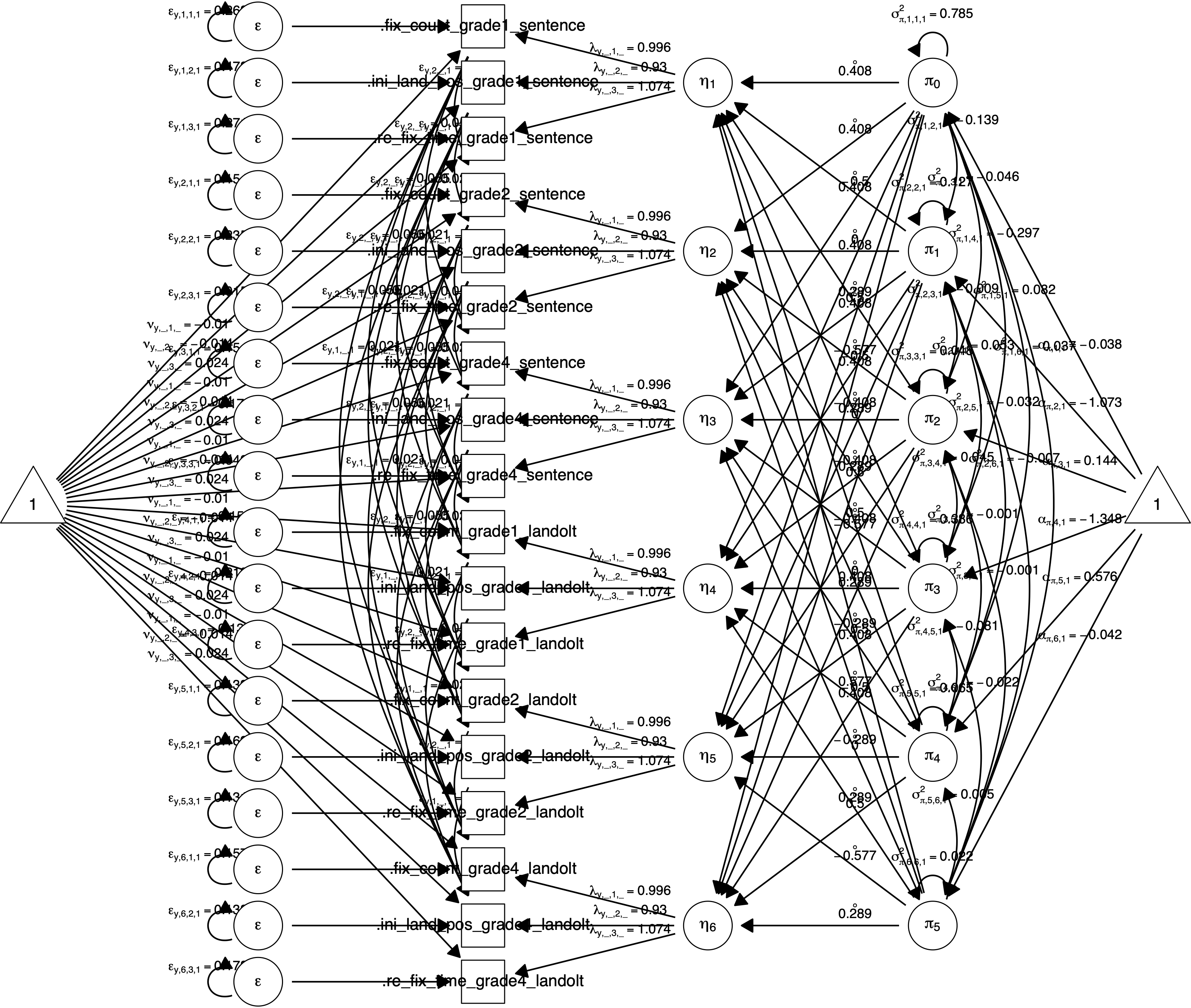
Figure 3.3: Path diagram created by plot(fit_latent, what = "all") for a \(2 \times 3\) (sentence \(\times\) grade) within-subjects design with the latent dependent variable reading ability measured by the three manifest variables re-fixation time, initial landing position and fixation count.
3.2.2 Measurement Invariance
Measurement invariance is an important assumption when using latent variables. This assumption is oftentimes implicitly assumed when using traditional repeated measures (RM-ANOVA). RM-ANOVA cannot handle latent variables and indicators are averaged to manifest composite or sum scores in order to be able to use RM-ANOVA. This approach implicitly assumes a parallel measurement model across the six experimental conditions but the assumption is not explicitly tested. In order to be able to compare the means of latent variables, we need strong measurement invariance (see Langenberg, 2022, sec. 2.4 “Latent Repeated Measures ANOVA (L-RM-ANOVA)”), that is, equal loadings and equal intercepts across the experimental conditions. With semnova, we can actually test for measurement invariance. As described in the previous example, semnova uses a congeneric measurement model. The invariance_within argument can be set to either of "configural" (equal model structure), "weak" (equal loadings), "strong" (equal loadings and intercepts), or "strict" (equal loadings, intercepts and residual variances):
fit_latent_configMI <- semnova(
    data = reading_latent,
    id = "id",
    dv = "dv",
    indicator = "indicator",
    equal_resid_cov = list("ini_land_pos", "fix_count"),
    within = c("grade", "sentence"),
    missing = "fiml",
    invariance_within = "configural"
)

fit_latent_weakMI <- semnova(
    data = reading_latent,
    id = "id",
    dv = "dv",
    indicator = "indicator",
    equal_resid_cov = list("ini_land_pos", "fix_count"),
    within = c("grade", "sentence"),
    missing = "fiml",
    invariance_within = "weak"
)

fit_latent_strongMI <- semnova(
    data = reading_latent,
    id = "id",
    dv = "dv",
    indicator = "indicator",
    equal_resid_cov = list("ini_land_pos", "fix_count"),
    within = c("grade", "sentence"),
    missing = "fiml",
    invariance_within = "strong"
)

fit_latent_strictMI <- semnova(
    data = reading_latent,
    id = "id",
    dv = "dv",
    indicator = "indicator",
    equal_resid_cov = list("ini_land_pos", "fix_count"),
    within = c("grade", "sentence"),
    missing = "fiml",
    invariance_within = "strict"
)

anova(
    fit_latent_configMI,
    fit_latent_weakMI,
    fit_latent_strongMI,
    fit_latent_strictMI
)
## Chi-Squared Difference Test
##
## Df AIC BIC Chisq Chisq diff Df diff Pr(>Chisq)
## fit_latent_configMI 118 5467.5 5722.2 248.11
## fit_latent_weakMI 128 5579.8 5798.6 380.44 132.332 10 < 2.2e-16 ***
## fit_latent_strongMI 138 5640.9 5823.9 461.55 81.114 10 3.036e-13 ***
## fit_latent_strictMI 153 5875.1 6004.2 725.68 264.131 15 < 2.2e-16 ***
## ---
## Signif. codes: 0 '***' 0.001 '**' 0.01 '*' 0.05 '.' 0.1 ' ' 1Using the anova() function, we can compare the four models. All tests are highly significant indicating that they do not fit equally well. Thus, we cannot assume any degree of measurement invariance. As a consequence, we should be very cautious when interpreting parameter estimates and hypothesis tests.