5 Covariates

The semnova() function can further incorporate manifest and latent covariates. The covariates argument takes a list of character vectors representing the variable names of covariates. If a character vector from the list consists of only one element, the covariate is treated as manifest, and as latent otherwise. If a manifest covariate points to a variable that contains a factor or characters, the variable will be dummy coded and included in the model. Interactions between manifest covariates will also be included. Interactions between latent covariates are not possible at this moment. Manifest variables measuring latent covariates must further be numerical.

In the next example, we estimate a $2 \times 3$ within-subjects design for re-fixation time and include sex as a dummy-coded covariate and the latent covariate child behavior measured at the end of the study by the two scales internalizing and externalizing behavior. The scales are taken from the child behavior checklist (CBLB, Achenbach, 1991).

fit_covariates <- semnova(
    data = reading_manifest,
    id = "id", 
    dv = "re_fix_time",
    within = c("grade", "sentence"),
    covariates = list("sex", CBCL = c("cbcl_int_verh_rw_t5", "cbcl_ext_verh_rw_t5"))
)

summary(fit_covariates)

## Fit measures:
## 
## Chisq(9) = 25.066, p = 0.003
## CFI = 0.962
## TLI = 0.847
## RMSEA = 0.107 [0.059, 0.158]
## 
## ##############################
## 
## Main and Interaction Effects:
##                       Chisq df Pr(>Chisq)    
## Intercept             1.105  1      0.293    
## grade               213.637  2     <2e-16 ***
## sentence            129.699  1     <2e-16 ***
## grade:sentence       57.760  2     <2e-16 ***
## sex                   0.002  1      0.964    
## grade:sex             2.263  2      0.323    
## sentence:sex          2.620  1      0.106    
## grade:sentence:sex    2.058  2      0.357    
## CBCL                  0.042  1      0.837    
## grade:CBCL            3.674  2      0.159    
## sentence:CBCL         0.257  1      0.612    
## grade:sentence:CBCL   2.648  2      0.266    
## ---
## Signif. codes:  0 '***' 0.001 '**' 0.01 '*' 0.05 '.' 0.1 ' ' 1

Residual covariances between re-fixation time and the internalizing and externalizing child behavior are fixed to zero which explains the nine degrees of freedom. The fit is not perfect but can be considered satisfactory because the confidence interval of the root mean squared error of approximation (RMSEA) includes the established threshold of 0.06 (e.g., Hu & Bentler, 1999). Hypothesis tests for within-subjects factors are again significant. Effects involving the covariate sex are non-significant which is in line with the multi-group model from the previous sections. Effects involving child behavior are also non-significant. That is, child behavior does neither predict differences between genders nor does it predict differences in re-fixation time between grades or sentence types. Figure 5.1 shows the path diagram of the model.

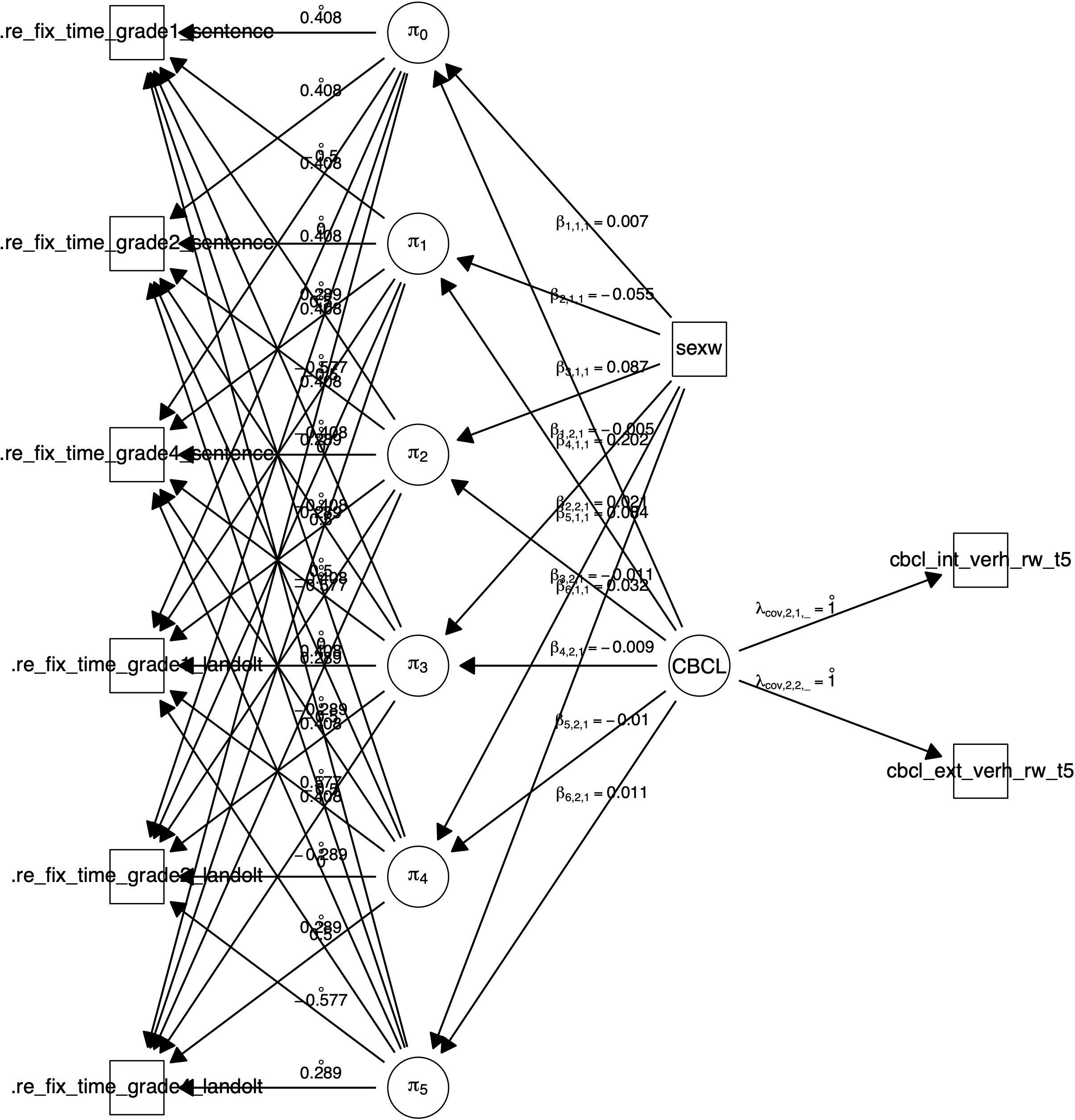
Path diagram created by `plot(fit_covariates)` for a $2 imes 3$ (sentence $ imes$ grade) within-subjects design with the manifest dependent variable re-fixation time, the manifest categorical covariate sex, and the latent covariate CBCL measured by the two manifest variables internalizing and externalizing child behavior.

Figure 5.1: Path diagram created by plot(fit_covariates) for a $2 imes 3$ (sentence $ imes$ grade) within-subjects design with the manifest dependent variable re-fixation time, the manifest categorical covariate sex, and the latent covariate CBCL measured by the two manifest variables internalizing and externalizing child behavior.