1 Motivating Example
The open-source R (R Core Team, 2021) software package semnova implements many of the methods demonstrated in this dissertation. The semnova package is based on the open-source R software package lavaan (Rosseel, 2012) which implements a wide range of methods for estimating structural equation models. This chapter gives an overview of the available features and explains the output by means of code examples using data from the motivating example about reading development in children from the introduction (see Langenberg, 2022, sec. 1.1.1 “Motivating Example”). Recall, in the study, \(N = 267\) children had to read two types of sentences: regular sentences or Landolt sentences in which characters are replaced by circles. The study included three measurements in the first, second, and fourth grade of school. Female and male children participated in the study. The dependent variables were re-fixation time1, initial landing position2, and fixation count3. The experimental design consists of a \(3 \times 2 \times 2\) mixed design, with the within-subjects factors grade (Factor A: A1 = grade one, A2 = grade two, A3 = grade four) and sentence type (Factor B: B1 = regular sentences, B2 = Landolt sentences). In this tutorial we additionally introduce the between-subjects factor sex (Factor C: C1 = female, C2 = male). Figure 1.1 shows the means and standard errors of re-fixation time, initial landing position, and fixation count across all six conditions for both genders. The data are included in the semnova package as a manifest and a latent version (reading_manifest and reading_latent). The data sets do not need to be explicitly loaded and can immediately be accessed after loading the package.
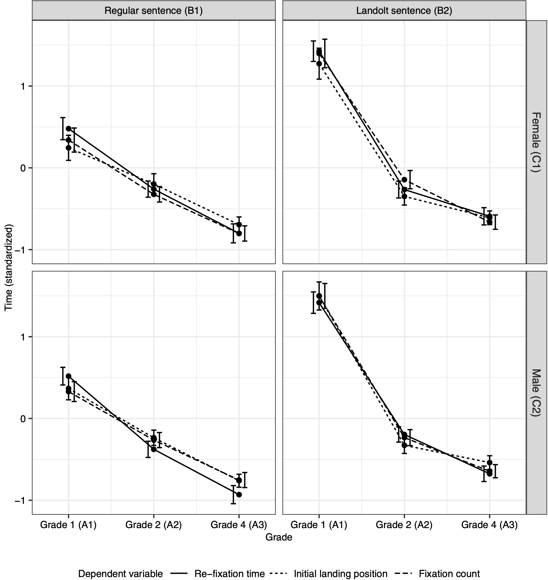
Figure 1.1: Re-fixation time (solid line), initial landing position (dotted line), and fixation count (dashed line) depending on sentence type (left panel: regular sentences; right panel: Landolt sentences), and sex (top panel: female; bottom panel: male) for the three measurement occasions (grade 1, grade 2, grade 4). The three variables were first averaged within children, then log-transformed and standardized. Shown are means across children. Error bars indicate standard errors.
We will use the same contrast matrix for the within-subjects design as in the introduction (see Langenberg, 2022, sec. 1.2 “Latent Repeated Measures ANOVA”). It is an orthogonal (i.e., linearly independent rows with length equal to one) polynomial contrast matrix and is given by:
\[ \mathbf{C} = \begin{pmatrix} 0.408 & 0.408 & 0.408 & 0.408 & 0.408 & 0.408\\ -0.5 & 0 & 0.5 & -0.5 & 0 & 0.5\\ 0.289 & -0.577 & 0.289 & 0.289 & -0.577 & 0.289\\ -0.408 & -0.408 & -0.408 & 0.408 & 0.408 & 0.408\\ 0.5 & 0 & -0.5 & -0.5 & 0 & 0.5\\ -0.289 & 0.577 & -0.289 & 0.289 & -0.577 & 0.289 \end{pmatrix} \tag{1.1} \]
In the following subsections, we will show numerous structural equation model (SEM) path diagrams that represent the estimated models. The entries from the inverse of the \(\mathbf{C}\) matrix (i.e. the \(\mathbf{B}^{*}\) matrix) can be found on the regression arrows from the \(\boldsymbol{\pi}\) variables to the \(\boldsymbol{\eta}\) variables. It is noteworthy that the inverse of the \(\mathbf{C}\) matrix equals its transpose because it is an orthonormal matrix. This is a convenient property because the regression coefficients from the path diagrams can be found in both the \(\mathbf{B}^{*}\) and the (``rotated’’) \(\mathbf{C}\) matrix. Thus, no inversion is needed to compare the path diagrams with the \(\mathbf{C}\) matrix.
Re-fixation time includes the total duration of fixations during the first gaze at a word excluding saccades in-between fixations. The variable is measured in milliseconds.↩︎
Initial landing position is the position of the letter of a word that was fixated first. The variable ranges from 0 to 6.↩︎
Fixation count is the number of fixations on a word during all gazes. The variable is a positive integer.↩︎