6 Power Analysis

The semnova package enables the researcher to perform power calculations for within- and between-subjects designs of any complexity. The power_script_semnova() function creates a script template making it very easy to specify population parameters in form of lavaan model syntax. The n_within argument takes an integer vector whose entries each represent a within-subjects factor with the number indicating the number of levels. n_between takes the same input for the between-subjects design. n_indicator takes a single integer representing the number of indicators. n_manifest_covariates takes the same input as n_within and n_between. However, if an entry equals one, the covariate is assumed to be continuous; if the entry is greater than or equal to two the covariate is assumed to be categorical with the number indicating the number of levels. n_latent_covariates take a vector of integers each representing a latent variable with the number indicating the number of manifest variables that measure the latent variable. Latent covariates are always assumed to be continuous. The sphericity argument takes a list of integer vectors and can be used to impose sphericity on effect variables of main or interaction effects. Each vector contains indices that refer to the within-subjects factors specified by n_within. out_file takes a path that the script file will be saved to.

What follows is an example for a $2 \times 3 \times 2 \times 2$ (within $\times$ within $\times$ between $\times$ between) mixed design with a latent dependent variable measured by three manifest variables, one continuous manifest covariate and one latent covariate measured by two manifest variables.

power_script_semnova(
    n_within = c(2,3),
    n_between = c(2,2),
    n_indicator = 3,
    n_manifest_covariate = c(1),
    n_latent_covariate = c(2),
    out_file = "power_script.R",
    sphericity = list(c(1,2))
)

The function will automatically name the factors, factor levels and covariates. Alternatively, the names can be given manually. The following code will produce exactly the same result as the previous example.

power_script_semnova(
    within = list(c(W = c("W1_1", "W1_2"), W2 = c("W2_1", "W2_2", "W2_3"))),
    between = list(c(B = c("B1_1", "B1_2"), B2 = c("B2_1", "B2_2"))),
    indicator = c("Y1", "Y2", "Y3"),
    manifest_covariate = c("covariate1"),
    latent_covariate = list(covariate2 = c("covariate2_1", "covariate2_1")),
    out_file = "power_script.R",
    sphericity = list(c("W1", "W2"))
)

Within-subjects factors are automatically given the prefix "W", between subjects factors have the prefix "B", covariates begin with the word "covariate", indicators of the dependent variables have the prefix "Y", indicators of the covariates start with the covariate name.

The function power_script_semnova() will create a script file that consists of three main parts. First, the script contains a lavaan model syntax that represents the specified model. The user has to replace parameter labels in the model syntax by population parameters. Second, the script contains a call to the power_analysis_semnova() function which will perform the power analysis and save the results to an object called power. The function takes the same input that was used to create the script file plus three additional parameters: data_syntax takes the lavaan model syntax containing the population parameters; sample_size takes a vector of sample sizes for the groups specified by the n_between or between (the length of the vector must be one or equal to the number of groups); replications takes the number of replications for the power analysis. Third, the three functions summary(), print(), and plot() are suggested to extract information from the resulting object. The following code is the result from the previous call to power_script_semnova saved to the specified output file.

data_syntax <- "
[...]
"

power <- power_analysis_semnova(
    n_within = c(2, 3),
    n_between = c(2, 2),
    n_indicator = 3,
    n_manifest_covariates = 1,
    n_latent_covariates = c(2),
    sphericity = list(2),
    data_syntax = data_syntax,
    sample_size = c(100, 100, 100, 100),
    replications = 500
)

# hypothesis tests
summary(power)

# parameters
print(power)

# path diagram
plot(power)

The contents of the data_syntax variable are omitted due to the large number of lines. The complete syntax can be found in Appendix A.

Appendix B further contains a copy of the previously created power script filled with example population parameters. Means of latent variables and regression coefficients are set to 0.1. Variances of latent variables are set to 1 and covariances to 0.5. Loadings of manifest variables are set to 1 and intercepts to 0. Residual variances are 0.4 and residual covariances are set to 0.

Depending on the number of replications and the complexity of the model, the power analysis may need some time to finish. After the analysis, the summary(power) function can be used to print a table that contains the power for the main and interaction effects of the model. In the following output, the results are truncated after the sixth hypothesis.

## Table: Hypotheses
## 
## hypothesis                    power
## -----------------------  ----------
## B1                        0.0456349
## B1:B2                     0.0456349
## B1:B2:covariate1          0.0357143
## B1:B2:covariate2          0.0634921
## B1:covariate1             0.0515873
## B1:covariate2             0.0595238
## [...]

We can further use the print(power) function to print the power and descriptive statistics for each of the model parameters separated by between-subjects factors (i.e., groups).

## Table: B1_1_B2_1
## 
## parameter                    mean          sd   pctNA       power       pct2.5        pct25       median       pct75     pct97.5
## --------------------  -----------  ----------  ------  ----------  -----------  -----------  -----------  ----------  ----------
## alpha_{pi,1,1}          0.0958489   0.1104171       0   0.1686508   -0.1392029    0.0188608    0.0999591   0.1698754   0.2996886
## alpha_{pi,2,1}          0.0977477   0.1118119       0   0.1666667   -0.1278233    0.0249539    0.0941303   0.1751148   0.3133758
## alpha_{pi,3,1}          0.0982346   0.1079209       0   0.1488095   -0.1170303    0.0220173    0.1044154   0.1701154   0.3070397
## alpha_{pi,4,1}          0.0994142   0.1099875       0   0.1428571   -0.1081087    0.0272029    0.1013290   0.1711141   0.3308732
## alpha_{pi,5,1}          0.1043942   0.1102061       0   0.1865079   -0.1095376    0.0330251    0.1028613   0.1854620   0.3055859
## alpha_{pi,6,1}          0.0997237   0.1035536       0   0.1329365   -0.0902241    0.0244948    0.1036009   0.1689088   0.2871981
## [...]

Lastly, the plot(power) function plots a path diagram for the model. The diagram will include parameter labels but no estimates.

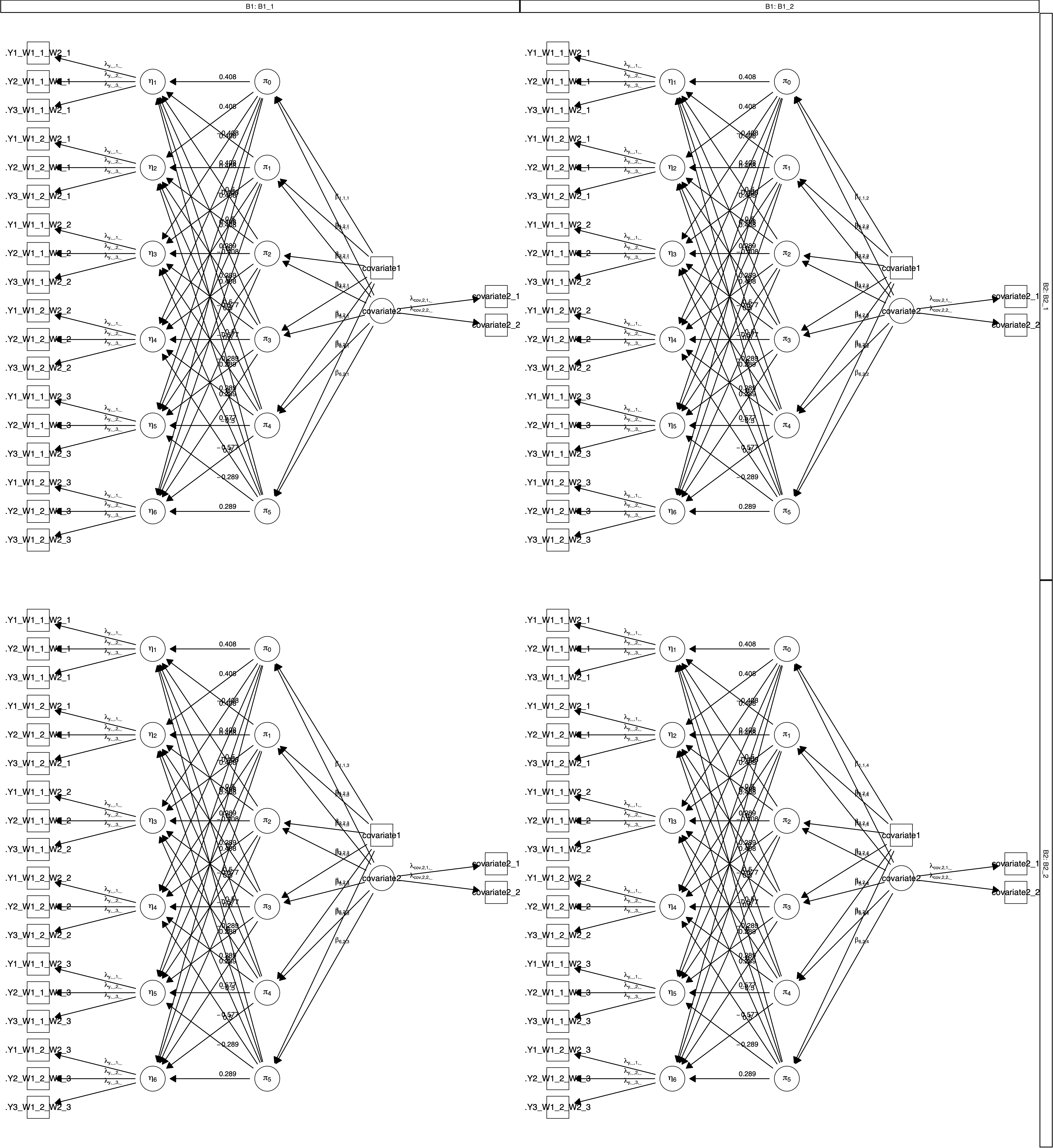
Path diagram created by `plot(power)` for a $2 imes 3 imes 2 imes 2$ (within $ imes$ within $ imes$ between $ imes$ between) mixed design with a latent dependent variable, one manifest covariates, and one latent covariate measured by two manifest variables.

Figure 6.1: Path diagram created by plot(power) for a $2 imes 3 imes 2 imes 2$ (within $ imes$ within $ imes$ between $ imes$ between) mixed design with a latent dependent variable, one manifest covariates, and one latent covariate measured by two manifest variables.